tensorboard可视化

Tensorboard导入与可视化图片
以手写数字分类mnist数据集为例：
下载mnist数据集，构造dataset：

train_ds = datasets.MNIST(
'data/',
train=True,
transform=transformation,
download=True
)
test_ds = datasets.MNIST(
'data/',
train=False,
transform=transformation,
download=True
)
1
2
3
4
5
6
7
8
9
10
11
12

查看mnist数据集包含的图片：

def imshow(img):
npimg = img.numpy()
npimg = np.squeeze(npimg)
plt.imshow(npimg)
plt.figure(figsize=(10, 1))
for i, img in enumerate(imgs[:10]):
plt.subplot(1, 10, i+1)
imshow(img)
1
2
3
4
5
6
7
8

导入tensorboard：
可视化两步骤：
1.在代码中将需要可视化的数据写入磁盘
2.在命令行中打开tensorboard，并指定写入的文件位置，进行可视化

from torch.utils.tensorboard import SummaryWriter

writer = SummaryWriter('my_log/mnist') # 指定写入位置
1
2
3
显示图片：

images, labels = next(iter(train_dl))

# create grid of images
img_grid = torchvision.utils.make_grid(images[-8:]) # 将多张图片合并在一起成一张图片
npimg = img_grid.permute(1, 2, 0).numpy()
plt.imshow(npimg)
1
2
3
4
5
6

写入图片到tensorboard：

writer.add_image('eight_mnist_images', img_grid)
1
在命令行窗口输入以下指令：

tensorboard --logdir=D:\PycharmProjects\PythonScript\Pytorch_Course_Study\my_log
1

打开给出的网址：http://localhost:6006/
查看到动态显示的图片：


模型网络结构的可视化
创建模型：

class Model(nn.Module):
def __init__(self):
super().__init__()
self.conv1 = nn.Conv2d(1, 6, 5)
self.pool = nn.MaxPool2d((2, 2))
self.conv2 = nn.Conv2d(6, 16, 5)
self.liner_1 = nn.Linear(16*4*4, 256)
self.liner_2 = nn.Linear(256, 10)
def forward(self, input):
x = F.relu(self.conv1(input))
x = self.pool(x)
x = F.relu(self.conv2(x))
x = self.pool(x)
# print(x.size()) # torch.Size([64, 16, 4, 4])
x = x.view(-1, 16*4*4)
x = F.relu(self.liner_1(x))
x = self.liner_2(x)
return x

model = Model()
1
显示模型：

writer.add_graph(model, images) # images为输入模型的数据
1
在tensorboard中查看模型：

双击model可查看模型内部结构：


标量数据的可视化
动态显示训练过程中的loss 和 acc的变化：

model.to(device)
loss_fn = torch.nn.CrossEntropyLoss() # 损失函数
1
2
使用write.add_scalar()方法：

def fit(epoch, model, trainloader, testloader):
correct = 0
total = 0
running_loss = 0
for x, y in trainloader:
x, y = x.to(device), y.to(device)
y_pred = model(x)
loss = loss_fn(y_pred, y)
optim.zero_grad()
loss.backward()
optim.step()
with torch.no_grad():
y_pred = torch.argmax(y_pred, dim=1)
correct += (y_pred == y).sum().item()
total += y.size(0)
running_loss += loss.item()

epoch_loss = running_loss / len(trainloader.dataset)
epoch_acc = correct / total

writer.add_scalar('training loss',
epoch_loss,
epoch)


test_correct = 0
test_total = 0
test_running_loss = 0

with torch.no_grad():
for x, y in testloader:
x, y = x.to(device), y.to(device)
y_pred = model(x)
loss = loss_fn(y_pred, y)
y_pred = torch.argmax(y_pred, dim=1)
test_correct += (y_pred == y).sum().item()
test_total += y.size(0)
test_running_loss += loss.item()

epoch_test_loss = test_running_loss / len(testloader.dataset)
epoch_test_acc = test_correct / test_total

writer.add_scalar('test loss',
epoch_test_loss,
epoch)


print('epoch: ', epoch,
'loss： ', round(epoch_loss, 3),
'accuracy:', round(epoch_acc, 3),
'test_loss： ', round(epoch_test_loss, 3),
'test_accuracy:', round(epoch_test_acc, 3)
)

return epoch_loss, epoch_acc, epoch_test_loss, epoch_test_acc

optim = torch.optim.Adam(model.parameters(), lr=0.001)
epochs = 20
train_loss = []
train_acc = []
test_loss = []
test_acc = []

for epoch in range(epochs):
epoch_loss, epoch_acc, epoch_test_loss, epoch_test_acc = fit(epoch,
model,
train_dl,
test_dl)
train_loss.append(epoch_loss)
train_acc.append(epoch_acc)
test_loss.append(epoch_test_loss)
test_acc.append(epoch_test_acc)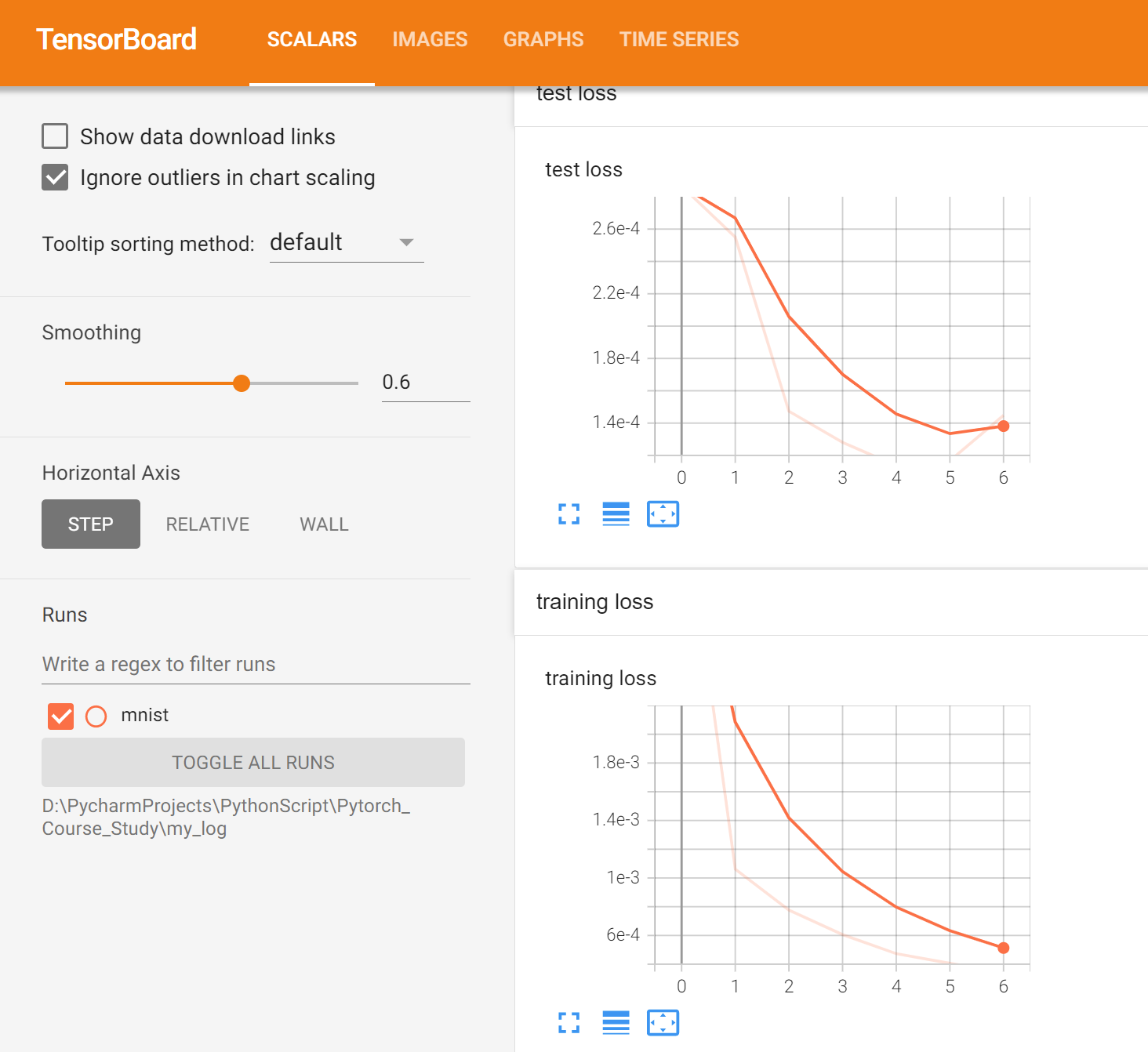

————————————————

版权声明：本文为博主原创文章，遵循 CC 4.0 BY-SA 版权协议，转载请附上原文出处链接和本声明。

原文链接：https://blog.csdn.net/qq_45850131/article/details/123920194